Behind the Data of the Virtual Cell Challenge

Authors: Yusuf H. Roohani, Alexander Dobin, Noam Teyssier, Basak Eraslan, Tony J. Hua, Po-Yuan Tung, Lexi R. Bounds, Abhinav Adduri, Alden Woodrow, Brian S. Plosky, Reshma Mehta, Benjamin Hsu, Jeremy Sullivan, Chiara Ricci-Tam, Nianzhen Li, Julia Kazaks, Luke A. Gilbert, Patrick D. Hsu, Silvana Konermann, Dave P. Burke, Hani Goodarzi

A high quality dataset to power the Virtual Cell Challenge

To enable meaningful model comparison in the Virtual Cell Challenge, we needed more than just a new Perturb-seq dataset; we needed a high-quality and high-fidelity benchmark. This required us to make careful decisions at every step: from perturbation strategy, to chemistry, to cellular context. Below we outline the key design principles and trade-offs that shaped the 2025 Virtual Cell Challenge dataset.

Choice of perturbation modality: dual-guide CRISPR-interference for targeted knockdown

CRISPR interference (CRISPRi) offers a powerful alternative to traditional CRISPR knockouts by repressing transcription without cutting the genome. Using a catalytically dead Cas9 (dCas9) fused to a KRAB transcriptional repressor, CRISPRi silences gene expression by targeting promoter regions, leaving the genomic sequence intact while sharply reducing mRNA levels (Gilbert et al. 2014). This feature makes CRISPRi especially well-suited for Perturb-seq since knockdown efficacy can directly be observed in the collected expression data (Replogle, Saunders, et al. 2022). In traditional CRISPR-Cas9 knockout experiments, where the protein-coding sequence is mutated, gene knockout isn’t always readily reflected in its mRNA levels.

Furthermore, we adopted a dual-guideRNA expression construct, where two guides targeting a gene of interest are simultaneously expressed from the same vector. This is to ensure strong and consistent knockdown across our target genes (Replogle, Bonnar, et al. 2022). Our experiments have shown that compared to single-guide designs, this dual-guide approach yields significantly improved and reliable depletion across genes.

Choice of chemistry: high-depth profiling with 10x Genomics Flex

To faithfully model how cells respond to perturbations, we need to observe gene expression changes with high resolution and minimal technical noise. We chose 10x Genomics Flex chemistry because it consistently produced the highest-quality data in our hands, both in pilot comparisons and in the full-scale screen. Before committing to a full run, we conducted a pilot experiment comparing standard 3’, 5’, and Flex chemistries on matched H1 embryonic stem cell (ESC) perturbations. Flex clearly outperformed both alternatives in UMI depth per cell, gene detection sensitivity, guide assignment, discrimination between perturbed and control cells.

Flex is a fixation-based, gene targeted probe-based chemistry for single-cell gene expression profiling. Unlike the standard 3’ or 5’ chemistries that rely on live-cell capture, poly-A tail priming, and reverse transcription, Flex enables transcriptomic profiling from fixed cells using targeted probes that hybridize directly to transcripts. This enables more uniform capture, better transcript preservation, removal of unwanted transcripts, capture of less abundant mRNAs, and the ability to scale deeply without sacrificing per-cell quality.

It is important to note that the probe-based quantification used with Flex requires a different data processing pipeline from most other methods, including our scRecounter pipeline (Youngblut et al. 2025).

Choice of cell type: human ESCs to test generalization

We deliberately selected H1 ESCs as the cellular model for this benchmark. Among human ESCs, H1 is the best characterized, and it is also included in ENCODE. Unlike previously profiled immortalized cell lines (like K562 or A375 cells), which dominate existing Perturb-seq datasets, the pluripotent H1 ESCs regulatory architecture, chromatin state, and response dynamics represent a true distributional shift relative to most public pretraining data. This choice was strategic: we wanted a dataset that requires models to generalize. By anchoring the benchmark in a cellular state poorly represented in the pretraining data, we avoid the risk that models succeed merely by memorizing response patterns seen in other cell lines.

Selection of target genes: capturing a spectrum of cellular responses

In parallel to our efforts in selecting the most appropriate chemistry for data generation, we also set out to construct a panel of 300 target genes that spans a wide spectrum of perturbation effects, from dramatic transcriptional shifts to nearly imperceptible ones, while ensuring coverage of biologically meaningful and diverse mechanisms.

We began with a large-scale CRISPRi pilot screen in H1 ESCs using dual-guide construct design, protospacer sequences and cloning strategy from (Replogle, Bonnar, et al. 2022). This gave us an empirical distribution of perturbation effects, measured as the number of differentially expressed (DE) genes per perturbation. From this, we binned perturbations based on the number of differentially expressed genes (i.e., perturbation strength). Each bin was sampled to maximize diversity in expression outcomes and to ensure the inclusion of both well-characterized and less-studied regulatory targets.

To avoid redundancy and ensure coverage of diverse cellular pathways, we applied ContrastiveVI+, a representation learning method, to the single-cell transcriptomes from the pilot screen. We then clustered perturbation responses in its latent space, ensuring that the final list of target genes included perturbations from all parts of this learned manifold. This strategy ensured that we captured diverse modes of response, not just genes that triggered a large number of differentially expressed genes (DEGs).

We included several additional relevant criteria in our selection as well: clean guide assignment, sufficiently high basal expression of the target gene (to ensure measurable knockdown), and strong target gene repression captured by Flex chemistry. We believe that this design allows for rigorous benchmarking of model sensitivity, specificity, and generalization across a realistic and heterogeneous set of biological challenges.

The Virtual Cell Challenge dataset is born

Having selected 300 target genes and their protospacer sequences, the cellular context, the CRISPR modality, and data collection strategy, we proceed to generate a high quality dataset for the Virtual Cell Challenge. The guide library was cloned in a similar manner as our pilot screen and validated for uniformity and coverage. For the large-scale Perturb-seq study, our CRISPRi H1 cells were transduced with lentivirus harboring the Virtual Cell Challenge guide library at low multiplicity of infection (MOI; to ensure single construct per cell), and maintained at high cell coverage throughout the entire experiment. In total, the dataset spans ~300,000 cells, all deeply profiled, strongly and uniformly silenced, and mapped to a clearly defined ground truth. The table below summarizes the key metrics.

	Value (median / mean)	Why it matters
Cells per perturbation	~1,000	Robust effect size estimates
UMIs per cell	> 50 000	Captures subtle transcriptional shifts impossible at shallow depth
Guides detection	63% of cells with both correct guides detected	Extremely low assignment errors
Knock-down efficacy	83% of cells with >80% knockdown	Confirms perturbations, not noise

Generating training/validation/test splits

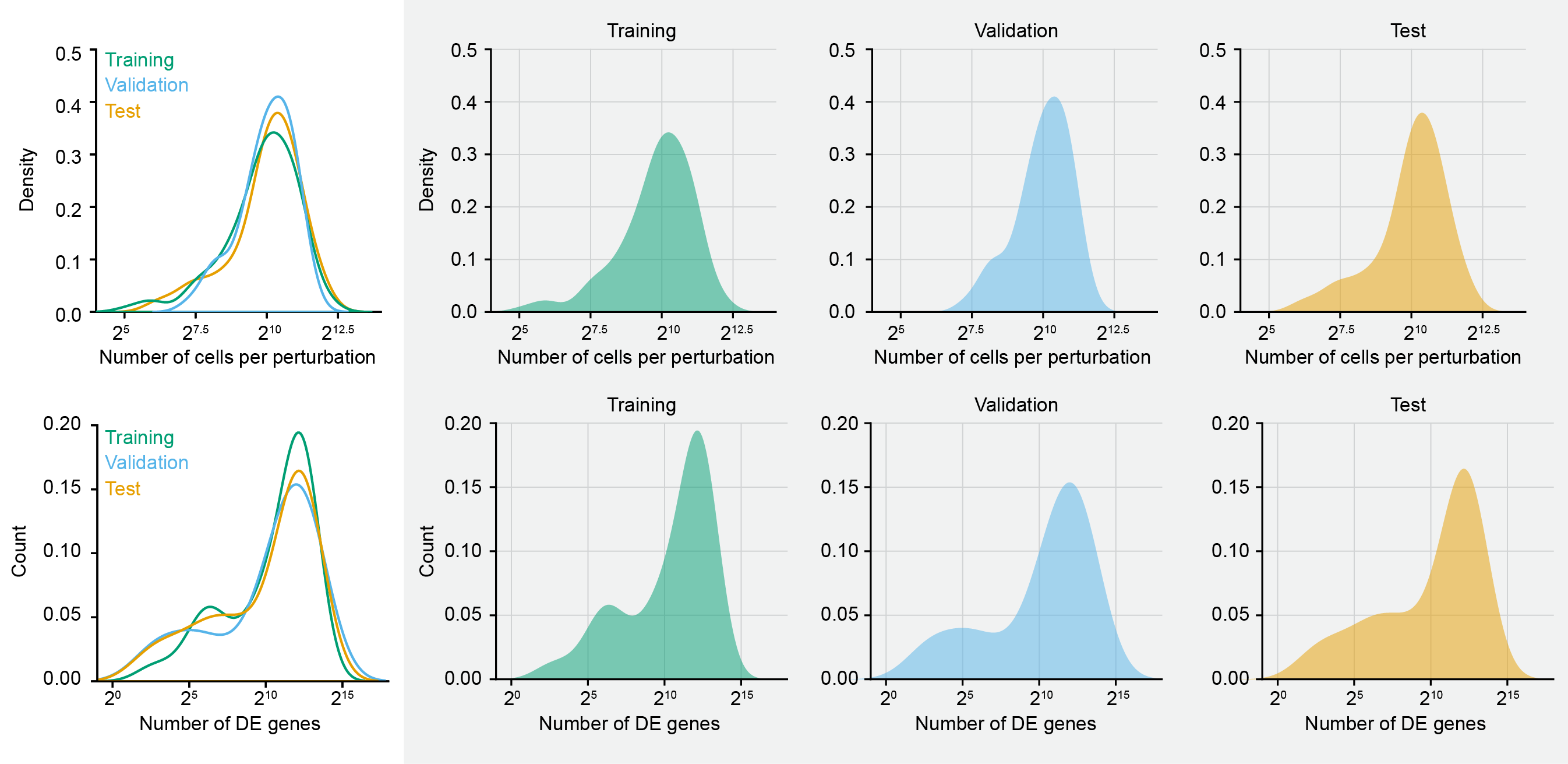
We calculated a stratification score for every targeted gene, taking into account both the number of differentially expressed genes and the number of high-quality assigned cells. This score served as a proxy for both biological signal strength and data richness. We then sorted the target genes by their stratification scores and divided them into bins representing different tiers of perturbation strength and quality. From each bin, target genes were randomly sampled into training, validation, and test sets, with a total of 150, 50, and 100 perturbations, respectively. This strategy ensured that all three data splits were compositionally balanced and drawn from the same underlying distribution, thereby mitigating concerns of out-of-distribution generalization. The resulting partition allows for a rigorous and unbiased assessment of model performance, where success on the validation and test sets reflects true generalization rather than sampling artifacts or distributional shifts.

Evaluation metrics in the Virtual Cell Challenge

What exactly constitutes a virtual cell is still an open question. But there’s growing consensus around one foundational capability: predicting how a cell’s state, as measured by its gene expression profile, changes in response to perturbation. In other words, the first true benchmark for a virtual cell is whether it can stand in for an actual experiment like Perturb-seq. In designing the Virtual Cell Challenge, we deliberately selected evaluation metrics that reflect how Perturb-seq is used by biologists in practice, not just how models perform on machine learning benchmarks. Biologists use these datasets to: (i) identify differentially expressed (DE) genes after perturbation, (ii) compare perturbation responses, and (iii) quantify transcriptional effects globally and at gene-level resolution.

Accordingly, our evaluation framework centers around three metrics that directly map to those practical use cases:

• Differential expression score (DES): captures whether the model recovers the correct set of differentially expressed genes.
• Perturbation discrimination score (PDS): measures whether the model assigns the correct effect to the correct perturbation (i.e. the predicted state is closest to the target perturbed state, relative to the other perturbations).
• Mean absolute error (MAE): assesses global expression accuracy across all genes.

In the sections below, we go into the details for calculating each metric and describe how they combine to produce the final leaderboard score.

Differential expression score

This metric evaluates whether a model can recover the correct set of differentially expressed (DE) genes after perturbation, based on statistical tests. For each perturbation $k$DE genes are called using a Wilcoxon rank-sum test between perturbed and control cells (on both predicted and true data). Significant genes are defined at FDR ≤ 0.05 using Benjamini-Hochberg correction. DE genes are then ranked by log fold-change (logFC) for both the ground-truth expression data and the model predictions, respectively.

Let:

• $G_{k,\text{true}}=$ set of significant DE genes in the ground truth
• $G_{k,\text{pred}}=$ set of significant DE genes in the prediction
• $n = |G_{k,\text{true}}|$

If $|G_{k,\text{pred}}| > |G_{k,\text{true}}|$, we select the top $n$ predicted DE genes by absolute log fold-change.

Score per perturbation is then calculated as: $\text{DES}_k = \frac{|G_{k,\text{true}} \cap G_{k,\text{pred}}|}{|G_{k,\text{true}}|}$, and the overall score:

$\text{DES} = \frac{1}{N} \sum_{k=1}^{N} \text{DES}_k$

This score ranges from 0 to 1 (higher being better).

Perturbation discrimination score

This metric tests whether a model's prediction for perturbation $p$ most closely resembles the correct ground truth profile among a pool of ground truth perturbations. For this score, we first construct pseudobulk profiles (average expression across cells) for each predicted and true perturbation. We then compute the perturbation delta ($\delta_{p}$) from non-targeting controls ($x$): $\delta_{p} = x_{p} - x$.

We then compute the L1 (Manhattan) distance between predicted perturbation delta $\delta_{p}$ and all ground truth pseudobulk deltas: $d_{pt} = || \hat{\delta^p} - \delta^t||_{1}$. We then rank the true perturbation $t=p$ in ascending order of distance (rank 1 = closest), and define the score as $\text{PDS}_p = 1 - \frac{r_p - 1}{N}$, where $r_p$ is the rank of the true match among all $N$ perturbations. The overall score for the model becomes:

$\text{PDS} = \frac{1}{N} \sum_{p=1}^{N} \text{PDS}_p$

This score ranges from 1 (perfect match) to ~0.5 (random guessing). In other words, PDS rewards perturbation-specific fidelity, especially for subtle phenotypes. Models predicting only global shifts or shared stress responses tend to have high DES but low PDS.

Mean Absolute Error (MAE)

This is an established metric that provides a global measure of reconstruction accuracy across the full transcriptome, regardless of statistical significance. The score for each perturbation is calculated as $\text{MAE}_k = \frac{1}{G} \sum_{g=1}^{G} \left| \hat{y}^k_g - y^k_g \right|$, where $G$ is the total number of genes, and $\hat{y}^k_g$ and $y^k_g$ are the predicted and true pseudobulk expressions for gene $g$. The overall score then becomes:

$\text{MAE} = \frac{1}{N} \sum_{k=1}^{N} \text{MAE}_k$

For MAE, lower is better, and there are no negative scores. It effectively captures prediction calibration and smoothness, even for non-DE genes. A trivial mean baseline that outputs the unperturbed average for every perturbation can perform surprisingly well on MAE but will fail on DES/PDS.

Final combined score

Each model is ranked on each metric independently. To produce a final leaderboard score:

• Each of the three metrics are normalized with respect to the perturbation-mean baseline to measure their performance gain over the naive baseline.

• A composite score is computed by taking the mean of the three normalized metrics.

• Minimum thresholds on each metric are enforced to prevent models from optimizing one at the expense of others.

• In addition, raw scores and per-perturbation breakdowns are made available to highlight different model behaviors. Notably we display the normalized metrics as we want to compare model performances to a naive but challenging perturbation-mean baseline.

  Metric	Measures	Range	Baseline Behavior
  DES	DE gene recovery accuracy	[0, 1]	High for models predicting common DEGs
  PDS	Perturbation-specific match	[0, 1]	Near 0.5 for trivial/random/constant predictions
  MAE	Global expression error	[0, ∞)	Low for models that ignore DEs but fit mean

The reality is that no single score (or even combination score) can capture the many nuances of perturbation prediction. As such, we have opted to show all scores on our leaderboard for the community to decide what matters to them in every application. Together, these metrics create a multi-axis evaluation framework that captures both biological relevance and quantitative performance. When it comes to virtual cell models, there is still an element of “we will know it when we see it” and as the field evolves, future challenges will likely expand this set of metrics.

We hope that pulling back the veil on the Challenge provides greater clarity for our choices of perturbation strategy, sequencing chemistry, cellular context, and metrics. In keeping with Arc’s practice of making datasets and models publicly available, we aim to be as transparent as possible with this and future Virtual Cell Challenges.

References

• Gilbert, Luke A., Max A. Horlbeck, Britt Adamson, Jacqueline E. Villalta, Yuwen Chen, Evan H. Whitehead, Carla Guimaraes, et al. 2014. “Genome-Scale CRISPR-Mediated Control of Gene Repression and Activation.” Cell 159 (3): 647–61. https://doi.org/10.1016/j.cell.2014.09.029.
• Replogle, Joseph M., Jessica L. Bonnar, Angela N. Pogson, Christina R. Liem, Nolan K. Maier, Yufang Ding, Baylee J. Russell, et al. 2022. “Maximizing CRISPRi Efficacy and Accessibility with Dual-sgRNA Libraries and Optimal Effectors.” eLife 11 (December). https://doi.org/10.7554/eLife.81856.
• Replogle, Joseph M., Reuben A. Saunders, Angela N. Pogson, Jeffrey A. Hussmann, Alexander Lenail, Alina Guna, Lauren Mascibroda, et al. 2022. “Mapping Information-Rich Genotype-Phenotype Landscapes with Genome-Scale Perturb-Seq.” Cell 185 (14): 2559–75.e28. https://doi.org/10.1016/j.cell.2022.05.013.
• Youngblut, Nicholas D., Christopher Carpenter, Jaanak Prashar, Chiara Ricci-Tam, Rajesh Ilango, Noam Teyssier, Silvana Konermann, et al. 2025. “scBaseCount: An AI Agent-Curated, Uniformly Processed, and Continually Expanding Single Cell Data Repository.” bioRxiv. https://doi.org/10.1101/2025.02.27.640494.

Note: On October 1, 2025, this post was updated to match the scoring methodology described in the STATE preprint.